ASAPprime® Data Analysis
Accurate, Predictive Data Analysis
Isoconversion
In traditional stability studies, degradation at fixed time points (e.g., 3, 6, 12, 18, 24 months) are determined. When higher temperatures are used, degradation is generally greater. The result is a different level of conversion at each condition.
When the degradation behavior of the product is not linear (the case in >60% of products), fitting of the data to temperature models is not predictive and is considered “non-Arrhenius.”
With ASAPprime®, data are analyzed in terms of isoconversion times at each condition. In this paradigm, the conversion to degradation products is kept constant to target the specification limit, while time is varied at each condition.
When degradation amounts at a particular condition are close to the specification limit, the estimation of the isoconversion time will have a small error bar. When extrapolation is needed, the precision will be lower.
ASAPprime® can fit the data to different curve shapes to best estimate isoconversion times. Normalized error bars for isoconversion times are calculated using error bars for the points themselves, typically a relative standard deviation (RSD) at higher degradation amounts and a fixed error at low degradation. Repeats and the quality of the fit are also factored into the probability calculations.
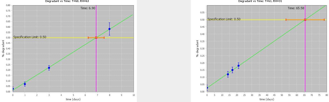
Screen shots of isoconversion plots for two conditions in an ASAPprime® study. In the example on the left, the isoconversion time (time to fail the specification limit) for the accelerated condition is determined by interpolation, and therefore has a relatively small error bar. In the example on the right, extrapolation was needed to estimate the isoconversion time, resulting in a larger error bar.
Modified Arrhenius Fitting
ln (1/t iso) = ln A – Ea/(RT) + B(RH)
A: collision frequency
Ea: activation energy
R: gas constant
T: temperature in Kelvin
B: humidity sensitivity factor
The isoconversion times (t iso) at all conditions are fit to the moisture-corrected Arrhenius equation above, which has been shown to work across all chemical and most physical changes that occur as samples age.
Instead of using rate constants, ASAPprime® uses the inverse of isoconversion times; error bars from the isoconversion times are propagated by Monte Carlo simulations to determine the precision in the fitting parameters. These are used to calculate the probability that a product will remain within its specification limits at the end of shelf-life.
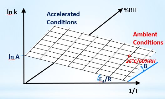
Graphical representation of the modified Arrhenius equation used with ASAPprime®.
ASAPprime® vs. Traditional Stability
In traditional stability programs, samples are analyzed as soon as they are removed from chambers. This leads to systematic error based on day-to-day offsets (instrument-to-instrument, analyst-to-analyst).
With ASAPprime®, samples, including the controls, are analyzed in a batch to minimize variability.
ASAPdesign™ can schedule when each sample should be added and removed from chambers.
To minimize any systematic error due to instrument drift or other causes, ASAPdesign™ provides a randomized order for analysis. This randomized order is especially important during comparison studies (e.g., formulation screening).
In traditional stability studies, wide latitude is allowed under the regulated conditions (e.g., 25±2°C/60±5%RH); however, with ASAPprime® studies, the actual measured conditions are used in the modeling.
The analytical results are reported even when nominally below the limit of quantitation (LOQ).

Example schedule for an ASAPprime® study where samples are put into chambers in a staggered order to allow all samples to be analyzed together at the final time.